A Recipe for Filtering Language Modelling Data

Some few weeks ago, I started a personal project to build a high-quality language modelling dataset from scratch.

When I used to hear people say they trained their model on "the internet", I thought all researchers built web crawler to source training data for their models. Turns out not, they use publicly available crawls. I decided to start with Common Crawl.

Looking into the raw data, it was mostly incoherent gibberish.

So I thought it could be useful to document the process of bridging the gap between this incoherent mesh and data I can train on. However, instead of just enumerating filtering steps, I want to dig a bit deeper and share the process I followed for developing a data pipeline. I share all the code I have written for this project here github repo.

I trained a GPT-2 small model on the data I curated for 200k step, and it achieved a validation score of "3.3" on C4 100 domains subset, this is a descent score and shows that following some simple steps and heuristics can lead to curating high quality data, although the engineering part was non-trivial.

The trick is to follow a certain methodology, one that, as far as I can tell, is not often documented. Let's start with two important observations that motivate it.

1. Public Web Data is a Leaky Abstraction

It is allegedly easy to get started with web-scale data. Numerous libraries and examples give the (false) impression that this stuff is plug-and-play. It's common to see things like:

>>> from datasets import load_dataset
>>> your_data = load_dataset("common_crawl", split="train")
# conquer world here

These one-liners activate the part of our brain that is familiar with clean software APIs.

Unfortunately, raw web data is nothing like that. It is not off-the-shelf technology.

Common Crawl doesn't just "give you" text. The pre-extracted text (WET files) is a mess of boilerplate, navigation menus, and cookie banners. The raw HTML (WARC files) is a full of broken tags, multiple languages, and programmatic spam.

2. Bad Data Fails Silently

When you break your model code, you often get an exception. An incorrect tensor shape. A failed import. A key not found.

This is just a start when it comes to data pipelines.

Everything can be syntactically correct, but the data itself can be fundamentally broken, and it’s really hard to tell. The "possible error surface" is huge and logical, not syntactic.

In my opinion, this error surface is motivated by one simple question, what makes good data ? this is a question I don't have an answer for yet, all I know now is how to make data "less bad".

For example, your dataset might be full of near-duplicates from templated websites. Your model can still train on this, but it will learn to memorize spammy patterns instead of generalizing. Or maybe your data is full of Personal identifiable information (PII), creating a major safety and privacy risk. Or the text is littered with leftover HTML tags and JavaScript snippets, teaching your model a broken form of language.

These are easy things to spot and deal with, the harder question is how to find the artifacts in a dataset that silently make your model a bit worse.

As a result, (and this is reeaally difficult to over-emphasize) a "fast and furious" approach to data filtering does not work and only leads to suffering.

Now, suffering is a natural part of building a good dataset, but it can be mitigated.

Part 1: The Recipe for Quality Data

In light of the above two facts, I have followed a specific process for filtering web data.

You will see that it takes the two principles above very seriously. It builds from simple to complex, and at every step, we make concrete hypotheses, validate them with experiments (i.e., by looking at the data), and investigate until we find the issue. What we try very hard to prevent is the introduction of a lot of "unverified" complexity at once, which is bound to introduce bugs and low-quality artifacts that will take forever to find.

Step 1: Become One with the Data

The first step to building a dataset is to not touch any filtering code at all. Instead, begin by thoroughly inspecting the raw source. This step is critical. I spent hours downloading random WARC and WET files from Common Crawl, just scrolling through them. What does the average page look like? (Answer: terrible). What kind of noise is most common? (Answer: navigation bars, ads, legal disclaimers, and cookie banners). How much non-English content is there? How much code?

Luckily, your brain is pretty good at this. I quickly realized the pre-extracted WET files was good enough; but I still wanted to have more control, so I started from the raw WARC HTML. I saw fragmented tags, endless lines of whitespace, and most text that was clearly not the "main content." This qualitative understanding is what informs the entire architecture of the pipeline. If your filters later produce something that doesn't seem consistent with what you’ve seen in the raw data, something is off.

Once you get a qualitative sense, write simple code to search and sort. In my case, this meant setting up a robust HTML-to-text extractor (resiliparse is great) and dumping the output to text files to see how well it worked.

Step 2: Set up the End-to-End Filtering Skeleton + Get Dumb Baselines

Now that we understand our data, can we build a fancy multi-stage filtering pipeline with parallel processing? For sure no. That is the road to suffering. Our next step is to set up a skeleton of the full process and gain trust in its correctness on a small scale.

At this stage, pick one single WARC file and make your goal to process it perfectly. We’ll want to apply a few simple filters, visualize the output at each stage, and perform a series of ablations with explicit hypotheses.

Tips & tricks for this stage:

Simplify. Turn off anything fancy. Just extract the text. My first pass simply used resiliparse to convert HTML to text. My baseline was seeing what came out. The key discovery here was that using its main_content=True flag dramatically improved the signal-to-noise ratio.
Log everything. Don't just output clean text. Your pipeline should output structured data, like a .jsonl file. For every document, save the text, the URL, the language detected by your next filter, its confidence score, etc. This metadata is your debugging lifeline.
Visualize the data at every step. The unambiguously correct way to verify a filter is to look at its input and output. I dumped random samples of text before and after language identification, before and after PII masking. This is the only "source of truth." I can’t count the number of times this revealed that my regex was too greedy or my whitespace normalization was breaking something.
Verify your filters on known examples. Find a web page with an email address. Does your PII filter catch it? Find a non-English page. Does your language ID filter catch it? Be your own unit test.
Overfit one file. Before you process petabytes, make your pipeline work perfectly on a single 1GB WARC file. Get the filters right, get the logic right, and ensure the output is exactly what you expect. If you can't get it right on one file, you have no hope of getting it right on one million.

Step 3: Overfit (on Quality)

At this stage, we have a pipeline skeleton that we trust. We can reproducibly take a raw $WARC$ file and produce a $JSONL$ file with structured, extracted text. Now, we want to get a model large enough that it can overfit. In our case, this means adding a set of aggressive filters to drive the "junk rate" as low as possible.

A few tips & tricks for this stage:

Don't be a hero. When it comes to filtering, my #1 advice is: find what has worked for others. I started by implementing the heuristic-based quality rules from the Gopher paper. They are simple and effective. I removed documents that were too short or too long, had weird word lengths, or too many non-alphabetic characters. Don't invent your own exotic quality metric at this stage.
Add one thing at a time. My pipeline evolved in discrete steps.
1. Language ID: Added fastText to keep only English. Result: ~75% of docs were filtered out.
2. Harmful Content: Added fastText classifiers for NSFW and hate speech. I set a high threshold (0.95) to be conservative. Result: Kept data dropped from 25.25% to 23.98%. In my case it was very rare to find documents that were false negatives for both toxicity and NSFW, but probably ensembelling or some heuristics like those used in Google's SafeSearch would be needed in high-stake training runs.
3. Gopher Rules: Added the heuristic filters. Result: Kept data dropped from 23.98% to a mere 9.86%. By adding filters sequentially and measuring the impact, you can understand what each component is doing. Throwing the kitchen sink at the data from the start is a recipe for confusion.
Track your work. The reason I can quote those exact percentages is because I logged them. For every filter, I tracked how many documents it removed. This helps you understand which filters are doing the heavy lifting.

More Quality filtering and PII:

The kept documents from the previous stages are hopefully not dangerous but the quality is far from guaranteed.

To add an additional safe guard, I trained a dedicated fastText classifier on labelled examples of "good" and "bad" web pages to learn a more nuanced quality signal.

For the positive samples, I used the data from Paloma C4 subset and scrapped URLs of the reference pages from a recent Wikipedia dump. I applied the previous pipeline to all of these document (in addition to the regularize part below).

For the negative samples I used random pages from Common Crawl. I trained the model using the fasttext library and quantized the resulting model to keep size small. Result: Kept data dropped from 9% to 3%

Finally, the surviving documents are masked for Personal identifiable information, mainly emails, phone numbers (which proved tricky to capture), and IP addresses.

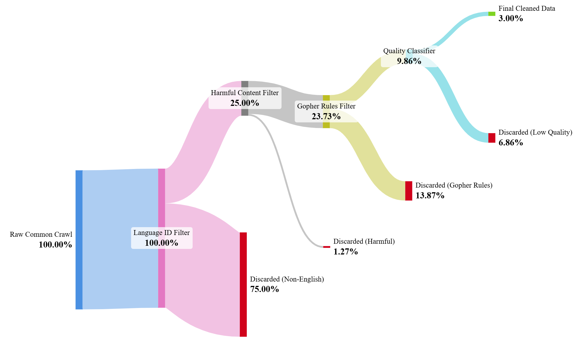
Figure 1: Sankey diagram that summarizes the filtering pipeline.

Step 4: Regularize

We now have a pipeline that produces (hopefully) high-quality text. But the web is massively redundant. We need to "regularize" our dataset to prevent our future model from just memorizing common sentences and documents. This means giving up some of our training data (the duplicates) to improve validation performance (generalization). .

Exact Deduplication. The simplest approach that works is to remove duplicate lines. I hash every single line of text across the entire dataset and keep only lines that appear exactly once. This is a brutal but effective way to remove boilerplate like "Copyright 2025," navigation links, and other low-effort spam.
Fuzzy Deduplication. For near-duplicates (e.g., the same article posted on two different sites), I use MinHash LSH. The intuition is simple: we create a compact "fingerprint" (MinHash) for every document. Then, we use a clever indexing trick (Locality-Sensitive Hashing) to only compare documents that are likely to be similar, avoiding the $O(n^2)$ nightmare. Finally, for the candidate pairs, we calculate the true Jaccard similarity and discard documents above a threshold (e.g., 85%), Implementation details are in the repository with more theory.

Step 5: Tune and Finalize

Once you have this entire pipeline, the final step is to tune it. This means tweaking the language confidence threshold, the Jaccard similarity threshold, or the Gopher rule parameters. The best way to do this is not a blind grid search, but an iterative process of changing one parameter, filtering a sample, and looking at what you kept and what you discarded.

In my final pipeline, I incorporated several additional heuristics:

Blacklist Filtering: I removed all lines that contain words from a pre-determined blacklist (e.g., navbar, cookies, lorem ipsum).
Line Length Filtering: I removed lines that contain less than five words.
AI Content Heuristics: I added a rule to remove documents with an excessive number of em dashes, a common artifact of some generative models.
Upranking Quality: I duplicated documents with the highest quality scores to increase their representation in the final dataset.

Part 2: Engineering a Scalable Pipeline

The recipe above defines what to do, but executing it on terabytes of data is an engineering challenge.

To make this practical, I broke the entire workflow into a three-stage pipeline. Each stage is a separate, runnable script with a clearly defined purpose, designed to manage a specific resource bottleneck: CPU, RAM, or I/O.

I managed to process 4000 WET files on my small local machine and modest internet speed.

Stage 1: Asynchronous Download & Filtering

The Goal: Asynchronously download massive WET files, run them through the heavy CPU-bound filters (language ID, harmful content, quality heuristics), and write only the surviving documents to disk.

The Challenge: You are I/O-bound from downloading hundreds of gigabytes, and simultaneously CPU-bound from running multiple ML models on the text.

A naïve approach where you download-then-process will leave your CPU idle. A simple parallel approach might load the multi-gigabyte FastText models into memory for every single file, crashing your machine instantly.

My Solution: I built a straightforward architecture to handle this.

An async I/O layer (aiohttp) acts as the quartermaster, managing hundreds of concurrent downloads efficiently without blocking. It writes incoming data to temporary files on disk, I controlled the peak storage usage with a semaphore on the maximum concurrent downloads.
A CPU worker pool (concurrent.futures.ProcessPoolExecutor): Each worker process loads the three FastText models once upon initialization, and applies the full filtering pipeline we detailed above.
The hand-off is simple but effective: the async layer downloads a file and passes its path to a worker process. The worker does its heavy filtering and returns a list of manifest entries for the documents that survived. This minimizes data transfer between processes.

I built in fine-grained controls for everything: max concurrent downloads, TCP connection limits, and number of CPU workers. This lets us tune the pipeline to the specific constraints of the machine.

Stage 2: Deduplication at Scale

The Goal: Take the millions of small text files from Stage 1 and perform both exact-line and fuzzy document-level deduplication.

The Challenge: Deduplication is fundamentally a global operation. To know if a line is a duplicate, you have to see all other lines. To find near-duplicate documents, you need to compare every document to every other document. Doing this in memory is impossible. You'd need hundreds of gigabytes of RAM.

Our Solution: I turned to SQLite. Instead of a complex distributed system or memory-hungry data structures, I used a central SQLite database on disk as the shared "brain" for the parallel workers.

Exact-Line Deduplication: I did this in two passes. First, worker processes chunked through all the documents, computed a SHA256 hash for every line, and wrote these hashes to a central SQLite table, incrementing a counter. Thanks to SQLite's WAL-mode, multiple workers could write concurrently without corrupting the database. In the second pass, workers re-read the documents, looked up each line's hash in the now-complete database, and only wrote out lines whose global count was 1.
Fuzzy Deduplication (MinHash LSH): I followed the same principle. Workers generated MinHash signatures for each document and stored them in a SQLite table. Then, the LSH banding logic was also performed by querying this database to find candidate pairs.

Using a file-based database as my synchronization primitive allowed me to solve a massive state-management problem with surprising simplicity and robustness, keeping the RAM footprint of each worker minimal.

To make this section more concrete, I would like to share with you some small code snippets that detail how I approached exact line deduplication.

The main function is as follows:

def exact_line_dedup_parallel(
    list_paths: List[str],
    output_directory: Path,
    num_workers: int | None = None,
    db_dir: Path | None = None,
)

We take a list of paths where each path points to a document, we also receive an output directory to write back each file, number of workers and path to the sqlite3 database directory.

This function has two main parts we can do in parallel, the local hashes counting and writing unique lines.

We will start with local hashes counting:

def local_hashes_counter(path: str):
    global _db_cur, _db_conn
    batch = []
    BATCH_SIZE = 5000

    def flush(batch_rows):
        if not batch_rows:
            return
        _db_cur.executemany(
            """
            INSERT INTO hash_cnt(hash, cnt) VALUES(?, 1)
	        ON CONFLICT(hash) DO UPDATE SET cnt = cnt + 1;
	        """,
            batch_rows
        )
    with open(path, "rb") as f:
        for line in f:
             batch.append(
                    (hashlib.sha256(line.strip()).hexdigest(),)
                  )
            if len(batch) >= BATCH_SIZE:
                flush(batch)
                batch.clear()
            flush(batch)

The logic is straightforward, we go through each line, hash it and add it to a table hash_cnt, on conflict, meaning when we have another line with the same hash, we increase the count.

We populate a batch size and insert when it saturates to keep memory in bound.

to launch this function we just call ProcessPoolExecutor:

with ProcessPoolExecutor(
    max_workers=min(num_workers, 8),
    initializer=init_db_writer,
    initargs=(db_path,),
) as exe:
    for _ in tqdm(exe.map(local_hashes_counter, list_paths, chunksize=32),
              total=len(list_paths)):
        pass

We pass init_db_writer as an initializer, it sets up the database connection for each worker and enables Write-Ahead Logging (WAL), which is crucial for allowing concurrent writes from multiple processes. and creates the hash_cnt table if it doesn't exist.

def init_db_writer(db_path: str):
    global _db_conn, _db_cur
    _db_conn = sqlite3.connect(db_path, check_same_thread=False, isolation_level=None)
    _db_cur = _db_conn.cursor()
    _db_cur.execute("PRAGMA journal_mode=WAL;")
    _db_cur.execute("PRAGMA synchronous=NORMAL;")
    _db_cur.execute("PRAGMA temp_store=MEMORY;")
    _db_cur.execute("CREATE TABLE IF NOT EXISTS hash_cnt(hash TEXT PRIMARY KEY, cnt INTEGER);")

Writing back unique lines follows the same pattern, and we just read from the table instead of inserting.

Stage 3: Final Tokenization

The Goal: Convert the final, clean, deduplicated text corpus into a single, compact binary file that can be memory-mapped for ultra-fast loading during model training.

The Challenge: This is a final, "embarrassingly parallel" CPU-bound task. The bottleneck is purely the speed of the tokenizer. We need to do this without loading the entire multi-gigabyte text file into memory.

Our Solution: This was the most straightforward stage, architecturally.

A single parent process reads the final text file line-by-line in a streaming fashion, ensuring a tiny memory footprint.
It deals out batches of lines to a ProcessPoolExecutor, where each worker has the GPT-2 tokenizer pre-loaded in memory.
Workers tokenize their batch of lines and return lists of uint16 token IDs.
The parent process simply receives these lists in order (guaranteed by executor.map) and writes their raw bytes sequentially to a single output file.

The final output is a flat binary file containing a concatenated stream of all tokenized documents. There are no delimiters, just pure token IDs. This format is perfect for training, as a framework can mmap the file and access any part of the dataset without reading the whole thing into RAM.

5. Training:

Finally, to validate the quality of the curated data, I used it to train a GPT-2 small model (124M parameters) for 200,000 steps

The training setup is conventional: DDP, AdamW and Cosine Annealing schedule.

The final evaluation perplexity on a 20k sample subset of the C4 validation set was 3.3.

For context, models of similar size trained on unfiltered or lightly-filtered web data typically plateau at a perplexity well above 10, demonstrating the significant impact of the curation pipeline.

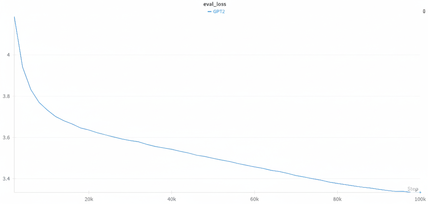Figure 2: GPT-2 Small (124M) training and evaluation loss curves.

Conclusion

Although my blog gives some rough advice on how to build a vanilla pipeline, it's in no way a production-grade setup, but it gives a good baseline for starting your data curation journey and ensures to some degree that the data you're about to spend tens of GPU-hours on isn't total garbage. Good luck!

References

Raffel, C., et al. (2020). Exploring the Limits of Transfer Learning with a Unified Text-to-Text Transformer. (The T5 paper, which introduced the C4 dataset).
Rae, J. W., et al. (2021). Scaling Language Models: Methods, Analysis & Insights from Training Gopher. (The Gopher paper you reference).
Joulin, A., et al. (2016). Bag of Tricks for Efficient Text Classification.
CS336: Assignment 4 2025 public repository